- Preparation: Standing on the Shoulders of Giants
- The Experiment
- Results - Architecture Comparison (5,000 steps)
- Results - Scaling Up
- Generated Names
- Key Findings
- Architecture Summary
- What the Loss Means
- Conclusion
After months of reading about transformers and LLMs, I finally decided to build one from scratch. Not by copy-pasting code, but by incrementally adding each architectural component and measuring its impact. The result was a character-level name generator trained on 32,033 names, and the journey taught me more than any paper or tutorial could.
Preparation: Standing on the Shoulders of Giants
Before diving into code, I spent time building intuition through two excellent resources:
“Build a Large Language Model (From Scratch)” by Sebastian Raschka was my theoretical foundation. The book walks through every component of a transformer with clear explanations and diagrams. Reading it gave me a mental model of how attention, embeddings, and layer normalization fit together — knowledge that proved essential when debugging my own implementation.
Andrej Karpathy’s YouTube series (Neural Networks: Zero to Hero) was equally valuable. His “Let’s build GPT” video demystified the architecture by building it live on screen. Watching someone think through the design decisions — why we use residual connections, how attention matrices work, what LayerNorm actually does — made the concepts stick in a way that reading alone couldn’t. His makemore repository became the dataset and benchmark for my experiments.
With this foundation, I was ready to build.
The Experiment
I incrementally built a character-level transformer for name generation. Each step adds one architectural improvement. All models were trained with batch size 32, AdamW optimizer, and per-name padding with masked loss.
Results - Architecture Comparison (5,000 steps)
| Config | N_EMBD | Heads | Layers | Params | Train | Test |
|---|---|---|---|---|---|---|
| baseline | 32 | 1 | 1 | 2,908 | 2.35 | 2.35 |
| double embd | 64 | 1 | 1 | 8,860 | 2.34 | 2.34 |
| 2 heads | 32 | 2 | 1 | 5,948 | 2.25 | 2.23 |
| 4 layers | 32 | 2 | 4 | 18,332 | 2.00 | 2.04 |
| + MLP | 32 | 2 | 4 | 51,740 | 1.97 | 2.02 |
| + LayerNorm | 32 | 2 | 4 | 52,252 | 1.96 | 1.99 |
| + RoPE | 32 | 2 | 4 | 52,252 | 1.94 | 1.98 |
| + GELU | 32 | 2 | 4 | 52,252 | 1.94 | 1.94 |
Results - Scaling Up
| Config | Steps | Train | Test | Notes |
|---|---|---|---|---|
| N_EMBD=32, 2 heads | 5,000 | 1.94 | 1.94 | Baseline final model |
| N_EMBD=64, 4 heads | 5,000 | 1.84 | 1.92 | Matches makemore architecture |
| N_EMBD=64, 4 heads + dropout | 5,000 | 1.95 | 2.00 | Dropout slows convergence |
| N_EMBD=64, 4 heads + dropout | 20,000 | 1.75 | 1.85 | Longer training helps |
| + LR schedule, weight decay, grad clip | 20,000 | 1.72 | 1.86 | Training improvements |
Makemore’s default transformer achieves ~1.92 test loss with N_EMBD=64, 4 heads, 4 layers.
Generated Names
Sample outputs from the final model (N_EMBD=64, 4 heads, 20k steps with all training improvements):
kaelynn, aileigh, elyce, yadi, ovani, derella, nyailee, ranyah, niaa, sett
Key Findings
Depth beats width
Doubling embedding size from 32 to 64 (3x params) gave almost no improvement (2.35 -> 2.34). Adding a second attention head with fewer total params (5,948 vs 8,860) dropped loss by 0.12. Stacking 4 layers was the single biggest improvement, dropping test loss from 2.23 to 2.04. The model benefits far more from multiple layers of processing than from wider representations at a single layer.
Data handling matters most
Before adding per-name padding, our best model achieved 2.36 test loss. After switching to per-name padding with masked loss (same architecture), it dropped to 1.94. This was a larger improvement than all architectural changes combined. The reason: without padding, the model wasted capacity trying to predict across name boundaries — an impossible task that added noise to every gradient update.
MLP adds capacity but needs regularization
Adding the feed-forward network (MLP) to each layer tripled the parameter count (18k -> 52k) but only modestly improved results. It also widened the train-test gap (2.00/2.04 -> 1.97/2.02), suggesting mild overfitting. The MLP lets the model transform representations nonlinearly after attention gathers information, but at this small scale the effect is limited.
LayerNorm and RoPE help incrementally
LayerNorm stabilized training and closed the train-test gap slightly. RoPE (Rotary Position Embeddings) gave the model awareness of character positions without adding any parameters. Neither was dramatic at this scale, but both are essential for larger models — LayerNorm enables training deep networks, and RoPE enables generalization to longer sequences.
GELU vs ReLU is negligible at small scale
Switching from ReLU to GELU activation in the MLP had no measurable effect. The smoother gradient flow matters more when networks are deeper and wider.
Scaling up helps significantly
Doubling N_EMBD to 64 and using 4 heads (matching makemore’s architecture) dropped test loss from 1.94 to 1.92 at 5k steps. With longer training (20k steps), the model reached 1.85 test loss — surpassing makemore’s default.
Dropout trades speed for generalization
Adding 20% dropout increased the train-test gap initially and slowed convergence. At 5k steps, it actually hurt test loss (1.92 -> 2.00). But it prevents overfitting during longer training runs, allowing the model to keep improving past where it would otherwise plateau.
Training improvements compound
Learning rate scheduling (warmup + cosine decay), weight decay (0.01), and gradient clipping (max_norm=1.0) together produced smoother training curves. The cosine decay prevents the learning rate from being too high in later steps when fine-tuning. Weight decay acts as regularization. Gradient clipping prevents instability from occasional large gradients.
Architecture Summary
The final model is a proper transformer decoder:
Input tokens
    -> Token Embedding (28 vocab -> 64 dim)
    -> 4x Transformer Blocks:
        -> LayerNorm -> Multi-Head Attention (4 heads, RoPE, dropout) -> Residual
        -> LayerNorm -> MLP (64 -> 256 -> 64, GELU, dropout) -> Residual
    -> Linear (64 -> 28 vocab)
    -> Cross-entropy loss (masked on PAD tokens)
Training config:
- 20,000 steps
- Batch size 32
- AdamW optimizer with weight decay 0.01
- Learning rate: warmup to 1e-3 over 200 steps, cosine decay to 1e-4
- Gradient clipping: max_norm=1.0
- Dropout: 0.2
What the Loss Means
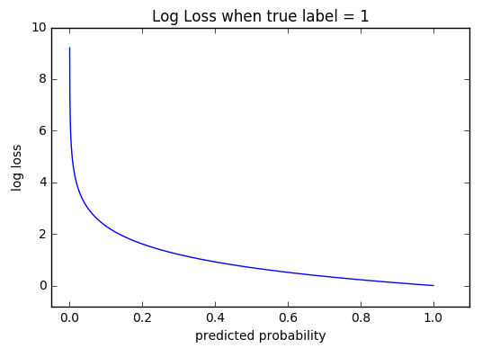
A loss of 1.86 means the model assigns ~15.6% probability on average to the correct next character (e^(-1.86)). Random guessing over 27 characters would give ~3.7% (loss = 3.30). Perfect prediction is impossible because many positions are genuinely ambiguous — after “ma”, the next character could be r, d, k, x, t, and many others.
Progress through this project:
- Start: 2.35 test loss (~9.5% confidence)
- Final: 1.86 test loss (~15.6% confidence)
- Improvement: ~1.6x more confident on the correct character
Conclusion
Building a transformer incrementally taught me that the magic isn’t in any single component — it’s in how they work together. Data preprocessing had the biggest impact. Depth mattered more than width. And the “modern” improvements (LayerNorm, RoPE, GELU) are less about dramatic gains and more about enabling scale.