- The Architecture: Encoder-Decoder with Cross-Attention
- From Pixels to Patches: The Vision Encoder
- Cross-Attention: The Bridge Between Vision and Language
- Training on Flickr8k
- Results: What the Model Learned
- Model Statistics
- Key Learnings
- Improvement: Using Pretrained CLIP Encoder
- Improvement: Word-Level Tokenization
- Improvement: CLIP + GloVe Pretrained Embeddings
- What’s Next
- Code
After building a text-only transformer for name generation, I wanted to tackle something more ambitious: teaching a model to describe images. This post documents my journey building a minimal image captioning transformer that learns to generate captions like “a dog runs through the snow” from raw pixels.
Try the live demo! - The model runs entirely in your browser using ONNX Runtime Web.
The Architecture: Encoder-Decoder with Cross-Attention
Unlike the decoder-only transformer from my previous experiment, image captioning requires an encoder-decoder architecture. The key insight is that we need to process two different modalities (images and text) and connect them through cross-attention.
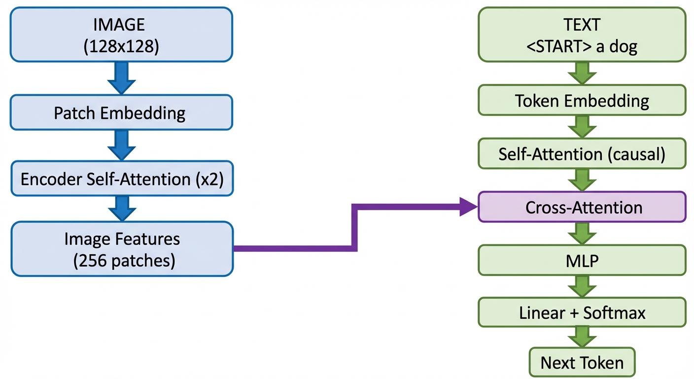
The architecture has two parallel paths:
Image Path (Blue): The image goes through patch embedding, then encoder self-attention layers. This produces “image features” — a sequence of patch embeddings that understand spatial relationships.
Text Path (Green): The caption tokens go through token embedding, then decoder layers with both self-attention (causal) and cross-attention to the image features.
The Bridge (Purple): Cross-attention is where the magic happens. It allows each text token to “look at” all image patches and gather relevant visual information.
From Pixels to Patches: The Vision Encoder
The first challenge is converting an image into something a transformer can process. Transformers work on sequences, but images are 2D grids. The solution: split the image into patches.
128x128 image → 16x16 grid of 8x8 patches → 256 patch embeddings
Each 8x8 patch contains 64 pixels × 3 colors = 192 values. A linear layer projects this to 128 dimensions:
class PatchEmbedding(nn.Module):
    def __init__(self, image_size, patch_size, n_embd):
        patch_dim = 3 * patch_size * patch_size  # 192
        self.proj = nn.Linear(patch_dim, n_embd)  # 192 → 128
        self.pos_embd = nn.Parameter(torch.randn(1, n_patches, n_embd))

    def forward(self, x):
        # Split image into patches, flatten, project
        patches = extract_patches(x)  # (B, 256, 192)
        return self.proj(patches) + self.pos_embd  # (B, 256, 128)
Now we have 256 “patch tokens” that can go through self-attention, just like text tokens. The encoder self-attention lets patches learn about each other — a patch showing a dog’s head can attend to patches showing its body and legs, building a coherent understanding of “dog”.
Cross-Attention: The Bridge Between Vision and Language
This is the key difference from text-only transformers. In self-attention, Q, K, and V all come from the same source. In cross-attention:
- Q (Query) comes from the text decoder: “What visual information do I need?”
- K, V (Key, Value) come from the image encoder: “Here’s what each patch contains”
class CrossAttention:
    def forward(self, text_embeddings, image_features):
        Q = text_embeddings @ W_q   # What am I looking for?
        K = image_features @ W_k    # What does each patch contain?
        V = image_features @ W_v    # What info to retrieve?

        scores = Q @ K.T  # (text_len, num_patches)
        weights = softmax(scores)
        return weights @ V  # Weighted sum of patch info
When generating the word “running”, the model learns to attend heavily to patches showing legs in motion. When generating “snow”, it attends to the white ground patches.
Training on Flickr8k
I used the Flickr8k dataset: 8,000 images with 5 human-written captions each. A key insight was using random caption sampling — each epoch, randomly select one of the 5 captions per image. This acts as data augmentation and dramatically reduces overfitting.
| Configuration | Train Loss | Val Loss | Notes |
|---|---|---|---|
| 64x64, fixed caption | 0.78 | 1.10 | Baseline |
| 128x128, fixed caption | 0.58 | 1.38 | More detail, more overfitting |
| 128x128, random caption | 0.90 | 0.99 | Much better generalization! |
The random caption sampling closed the train-val gap from 0.80 to just 0.09.
Results: What the Model Learned
After 30 epochs of training (~17 minutes on M4 Mac), the model generates reasonable captions:
Success case:
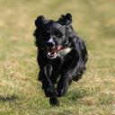
Generated: "a black dog is running through the grass ."
Actual:    "A black dog running across green grass ."
Failure case:

Generated: "a man in a blue shirt is standing in the stree"
Actual:    "A crowd of people are enjoying a meal with a view of a mountaintop ."
The model handles simple scenes well (dogs, people, basic actions) but struggles with complex scenes (crowds, multiple objects, subtle context).
Model Statistics
Total parameters: ~980,000 (about 1M)

Breakdown:
- Patch embedding:     32,896 (3%)
- Encoder blocks (2):  395,776 (40%)
- Token embedding:     8,960 (1%)
- Position embedding:  6,144 (1%)
- Decoder blocks (2):  527,616 (54%)
- Output layer:        9,286 (1%)
The decoder is larger than the encoder because each decoder block has both self-attention AND cross-attention.
Key Learnings
1. Patches are the “tokenizer” for images
Just as we split text into tokens, we split images into patches. This converts the 2D spatial structure into a sequence that transformers can process. The same weight matrix processes every patch, learning a universal “patch reader”.
2. Cross-attention is the bridge
The key architectural difference from text-only transformers. It lets the text generation process “see” the image at every step, attending to relevant patches for each word being generated.
3. Data augmentation matters enormously
Using all 5 captions with random sampling was more impactful than doubling the image resolution. The model learns semantic concepts rather than memorizing specific strings.
4. Resolution limits understanding
At 128x128, a tricycle looks like a blob. The model can distinguish dogs from people, but struggles with fine details. Real vision models use 224x224 or higher.
5. This is still a toy model
Production image captioning models use:
- Pretrained vision encoders (CLIP, ViT trained on millions of images)
- Word-level tokenization (shorter sequences)
- Much larger datasets (COCO has 330k images)
- Billions of parameters
Improvement: Using Pretrained CLIP Encoder
After training the from-scratch model, I wanted to see how much a pretrained vision encoder could help. I created a second version that uses CLIP ViT-B/32 as a frozen image encoder, training only the decoder and a projection layer.
Architecture Changes
Instead of learning patch embeddings from scratch:
- CLIP’s pretrained ViT processes the image (224x224 input)
- 50 patch embeddings (768-dim) are projected to the decoder dimension
- Only the decoder (~3.8M params) is trained; CLIP (~87M params) is frozen
class CLIPCaptioningModel(nn.Module):
    def encode_image(self, img):
        # Use CLIP's visual transformer (frozen)
        with torch.no_grad():
            x = clip_model.visual(img)  # (B, 50, 768)
        return self.visual_proj(x)  # Project to decoder dim
Results Comparison
| Metric | From-Scratch | CLIP-based |
|---|---|---|
| Val Loss | 1.29 | 0.86 |
| Train Loss | 1.23 | 0.75 |
| Epochs | 30 | 20 |
| Training Time | ~17 min | ~17 min |
| Model Size | 4 MB | 363 MB |
The CLIP-based model achieves 33% lower validation loss with fewer epochs!
Sample Captions
For the same test image (two dogs in snow):
| Model | Caption |
|---|---|
| From-scratch | “a black dog and a white dog are in the snow .” |
| CLIP-based | “two dogs playing in the snow .” |
| Ground truth | “a black dog is running after a white dog in the snow .” |
The CLIP-based model produces more natural, concise captions. It benefits from CLIP having been trained on 400 million image-text pairs — it already understands visual concepts like “dogs” and “playing” without needing to learn them from our small 8k image dataset.
Testing on Complex Scenes
I tested both models on the validation set, focusing on complex scenes that the from-scratch model struggled with:
| Scene | From-Scratch | CLIP-based | Ground Truth |
|---|---|---|---|
| Ice skating rink | “a man in a blue shirt…” | “a group of people standing in the snow .” | “A group of people are ice skating in a big city .” |
| Rock climbing | “a woman is standing…” | “a woman in a red shirt is climbing a rock .” | “A kid rock climbing against the backdrop of a green valley” |
| People at boats | “a man is…” | “a group of people standing in a rowd of a boat” | “A group of people waiting to ride boats .” |
| Mountain hikers | “a man in…” | “two people stand on the side of a mountain .” | “Three people facing the mountains .” |
Key observations:
- Better at groups/crowds — CLIP recognizes “group of people” much better than the from-scratch model which defaults to “a man”
- Better semantic understanding — Recognizes concepts like “rock climbing”, “mountain”, “boat” that the small model misses entirely
- Still struggles with fine details — Exact counts (two vs three people), specific activities (ice skating vs standing)
- More robust to complex scenes — Doesn’t collapse to generic “man in blue shirt” for difficult images
The pretrained visual features give CLIP a huge advantage on scenes requiring real-world knowledge.
Tradeoff: Accuracy vs Size
The improved model is 363MB (vs 4MB), making it impractical for browser deployment. This is the classic accuracy-size tradeoff:
- From-scratch model: Smaller, deployable, but less accurate
- CLIP-based model: More accurate, but requires a large pretrained encoder
For production, you’d typically use the large model on a server, or apply techniques like knowledge distillation to compress it.
Improvement: Word-Level Tokenization
The character-level model processes “a black dog” as 11 tokens (including spaces). Word-level tokenization reduces this to just 3 tokens, making sequences shorter and potentially easier to learn.
Parameter Count Changes
Switching from character-level to word-level tokenization dramatically changes where the parameters live:
| Component | Character-Level | Word-Level | Change |
|---|---|---|---|
| Token embedding | 8,960 (70 × 128) | 570,240 (4453 × 128) | +561K |
| Position embedding | 6,144 (48 × 128) | 2,560 (20 × 128) | -3.5K |
| Output layer | 8,960 | 570,240 | +561K |
| Total model | ~980K | ~2.1M | +1.1M (2.2×) |
The vocabulary explodes from ~70 characters to ~4500 words, but sequences shrink from 48 characters to 20 words. The net effect: 2.2× more parameters, almost entirely in the embedding layers.
Results Comparison
| Metric | Character-Level | Word-Level |
|---|---|---|
| Val Loss | 0.99 | 2.98 |
| Train Loss | 0.90 | 2.42 |
| Vocab Size | 70 | 4,453 |
| Max Seq Length | 48 | 20 |
| Model Size | 4 MB | 8.2 MB |
Wait — the word-level loss is higher? This is actually expected:
- Loss is per-token: Character-level predicts from 70 options; word-level predicts from 4,453 options
- Different scales: A word-level loss of 2.98 means perplexity ~20 (choosing from 4453 words), while character loss 0.99 means perplexity ~2.7 (choosing from 70 chars)
- The captions are similar quality despite the different loss values
Sample Caption
For the same test image (two dogs in snow):
| Model | Caption |
|---|---|
| Character-level | “a black dog and a white dog are in the snow .” |
| Word-level | “a dog is running through the snow .” |
| Ground truth | “a black dog is running after a white dog in the snow .” |
The word-level model produces fluent captions but with a smaller effective vocabulary (it saw each word fewer times during training than character-level saw each character).
Key Insight: Vocabulary Size vs Training Data
Word-level tokenization works better when you have lots of training data. With only 8k images:
- Character-level sees each character thousands of times → learns robust patterns
- Word-level sees many words only a few times → harder to learn good embeddings
This is why production models use:
- Subword tokenization (BPE, WordPiece): Best of both worlds
- Much larger datasets: COCO (330k), Conceptual Captions (3M+)
- Pretrained word embeddings: GloVe, Word2Vec, etc.
Improvement: CLIP + GloVe Pretrained Embeddings
Since the word-level model struggled with limited training data, I tried combining the best of both worlds: CLIP’s pretrained vision encoder with GloVe pretrained word embeddings.
The Idea
Instead of learning word embeddings from scratch with only 8k images, why not use GloVe embeddings trained on 6 billion words? This gives the model a head start on understanding word relationships.
class CLIPGloVeCaptioningModel(nn.Module):
    def __init__(self, vocab_size, clip_model, glove_embeddings, ...):
        # Use CLIP for vision (frozen)
        self.clip_model = clip_model

        # Use GloVe for word embeddings (fine-tuned)
        self.token_embed = nn.Embedding(vocab_size, glove_dim)
        self.token_embed.weight.data.copy_(glove_embeddings)

        # Project GloVe dim (100) to decoder dim (256)
        self.glove_proj = nn.Linear(glove_dim, n_embd)
GloVe Coverage
Using GloVe 6B 100d (100-dimensional embeddings trained on 6 billion tokens):
- 4441 out of 4517 words (98.3%) found in GloVe
- Only 76 words missing (mostly rare or domain-specific terms)
- Missing words initialized with small random values
Results
| Metric | Word-Level (random) | CLIP + GloVe |
|---|---|---|
| Val Loss | 2.98 | 2.55 |
| Train Loss | 2.42 | 1.78 |
| Epochs | 30 | 30 |
| GloVe Coverage | N/A | 98.3% |
The GloVe embeddings give a 14% improvement in validation loss!
Sample Caption
For the same test image (two dogs in snow):
| Model | Caption |
|---|---|
| Word-level (random init) | “a dog is running through the snow .” |
| CLIP + GloVe | “two dogs are playing in the snow .” |
| Ground truth | “a black dog is running after a white dog in the snow .” |
The GloVe model correctly identifies “two dogs” rather than “a dog”, suggesting the pretrained embeddings help with understanding quantities and relationships.
Key Insight: Transfer Learning Stacks
This experiment shows that transfer learning compounds:
- CLIP brings pretrained visual understanding (400M image-text pairs)
- GloVe brings pretrained word relationships (6B tokens)
- Only the decoder and projection layers need to learn task-specific mappings
Even with just 8k training images, combining two pretrained components achieves significantly better results than training from scratch.
What’s Next
Remaining improvements to explore:
Pretrained vision encoder: Use CLIP or ViT instead of learning from scratch✅ Done!Word-level tokenization: “a black dog” as 3 tokens instead of 11 characters✅ Done!Pretrained word embeddings: Use GloVe for better word representations✅ Done!- Subword tokenization: Use BPE for better vocab coverage
- More data: COCO dataset (330k images) instead of Flickr8k (8k)
- Knowledge distillation: Train a small model to mimic the CLIP-based one
But even the minimal from-scratch implementation demonstrates the core concepts: patch embeddings, encoder-decoder architecture, and cross-attention as the bridge between vision and language.
Code
The complete training script is available in my learn-llm repository as train-image-caption.py.